How to Find Relative Frequency in Excel
Fast navigation
In 4 very easy steps, this guide will show you how to find relative frequency in Excel.
Calculating relative frequency in excel is straightforward and easy to accomplish with these methods.
So let’s dive in and calculate relative frequency in Excel!
Steps:
- Open your Excel spreadsheet and enter your data
- Create the relative frequency formula
- Copy the formula to other cells
- Format the relative frequency values as percentages
Step 1: Open your Excel spreadsheet and enter your data
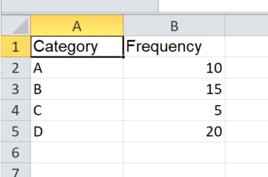
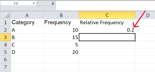
First, you need to input your data into the Excel spreadsheet. In column A, enter your categories or data points and in column B, enter the corresponding frequency values.
Step 2: Create the relative frequency formula
Now, you need to calculate the relative frequency for each data point.
The relative frequency is the individual frequency divided by the total of all frequencies.
Click on the cell next to the first frequency value (e.g., C2). Enter the formula: **=B2/SUM($B$2:$B$5)**
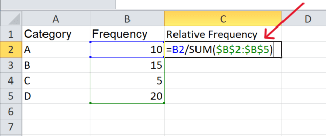
Here, B2 is the first frequency value, and SUM($B$2:$B$5) is the sum of all frequencies. The dollar signs lock the reference to the total sum, ensuring it doesn't change when copying the formula.
Press ‘Enter’, then you can see the first relative frequency in C2.
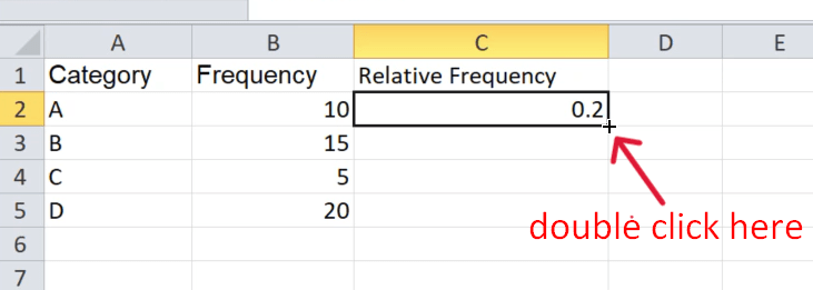
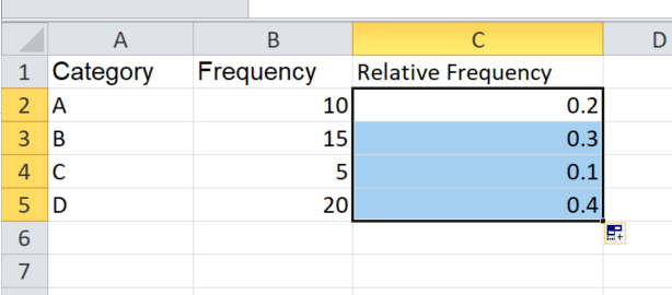
Step 3: Copy the formula to other cells
Step 4: Format the relative frequency values as percentages
To make the relative frequency values easier to understand, you can format them as percentages.
Select the cells with the relative frequency values (C2 to C5). Click on the "Percent Style" button in the toolbar (usually represented by a % symbol).
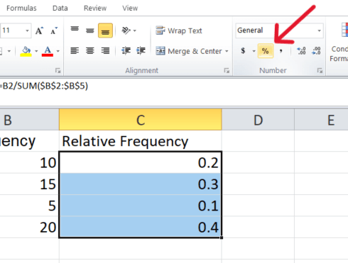
Now relative frequency values show as percentages.
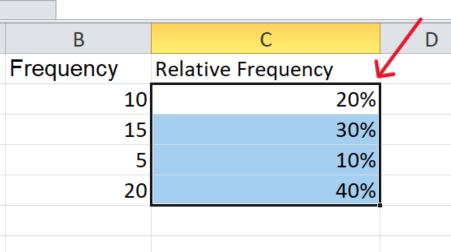
To show more decimal places for greater accuracy:
With the cells still selected, click on the "Increase Decimal" button in the toolbar.
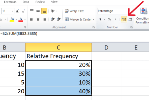
I rounded this up to two decimal places.
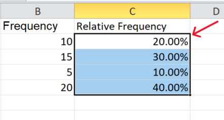
And that's it! You have successfully found and calculated the relative frequency for your data set in Excel.
By following these steps, you can easily compute and format relative frequencies for any data set, making your data analysis more insightful and informative.
Finished!

