All articles

How to Copy Only Visible Cells in Google Sheets

Last Updated: Fri Aug 16 2024

In 3 simple methods, this guide will show you how to copy only visible cells in Google Sheets.

Excluding hidden data ensures your datasets remain clean and relevant.

So let’s dive in and learn how to copy only visible cells in Google Sheets!

Method 1: Copy Only Visible Cells by Selecting Individual Ranges

This method is useful for datasets with hidden rows and columns.

Select the first range of visible cells by holding down the Ctrl key in your keyboard and clicking the cells you want to copy with the mouse.

Continue selecting additional visible ranges while holding down the Ctrl key.

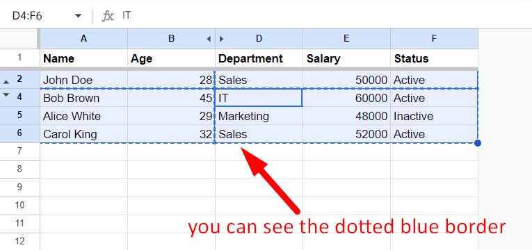
In the screenshot, I highlighted (A2:B2), (D2:F2), (A4:B6) and (D4:F6)

With the visible cells highlighted, press Ctrl + C to copy the data.

You should see a dotted blue border around the selected cells in your Google Sheet, indicating that only these cells are copied.

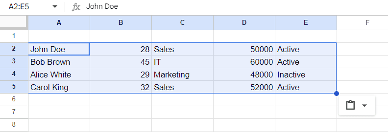
Navigate to the location where you want to paste the copied data and press Ctrl + V. Only the visible cells will be pasted in the new location.

Method 2: Copy Only Visible Cells with Grouped Rows and Columns

This method is ideal when dealing with grouped rows or columns.

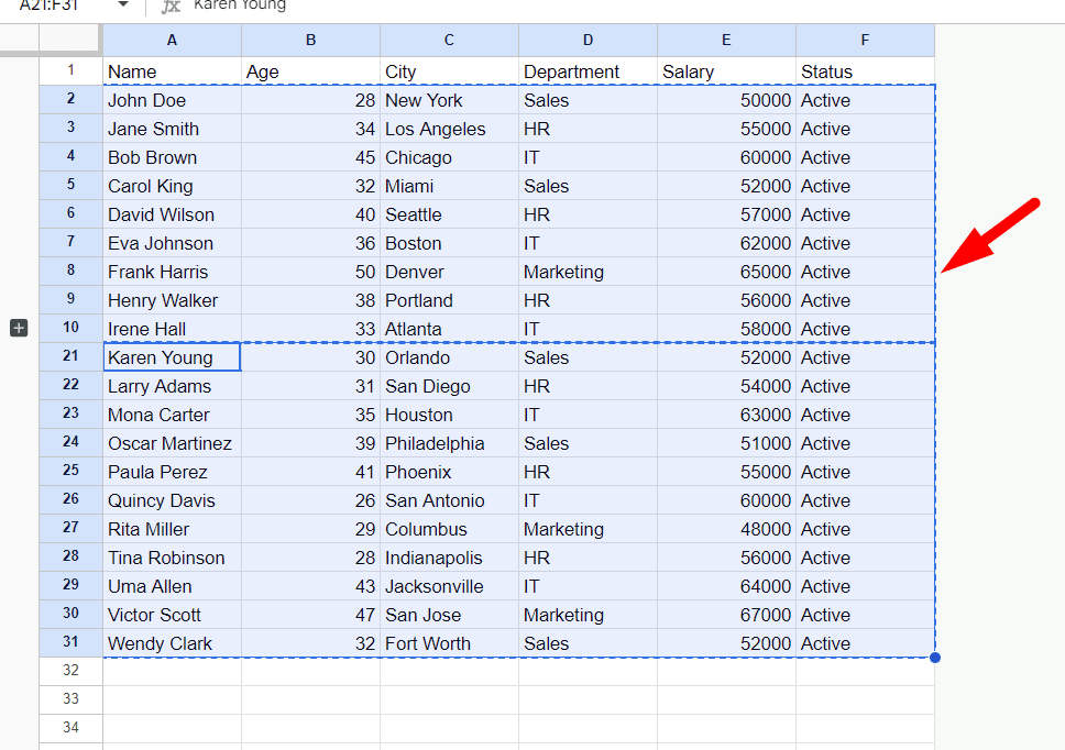
Use the Ctrl key to select the visible cells, ensuring you avoid the grouped rows or columns.

In the screenshot, row #11 - 20 are grouped.

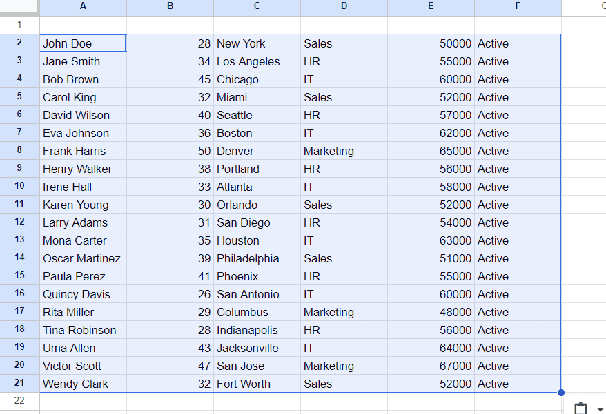
Follow the same copy and paste steps as above (Method #1) to ensure only the visible, ungrouped data is transferred.

Method 3: Copy Only Visible Cells with Filtered Data

This method is for when you’ve applied filters to your data and need to copy only the visible rows.

Apply your desired filter to the dataset to show only specific rows.

Select the filtered, visible rows and copy them using Ctrl + C.

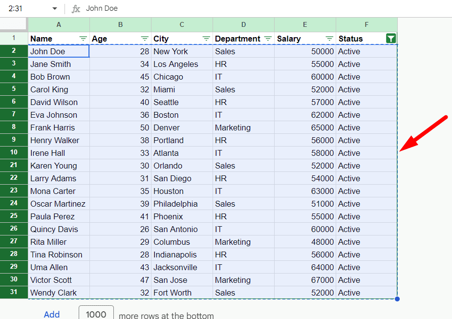
Paste the copied data where needed. Only the filtered, visible rows will be included.

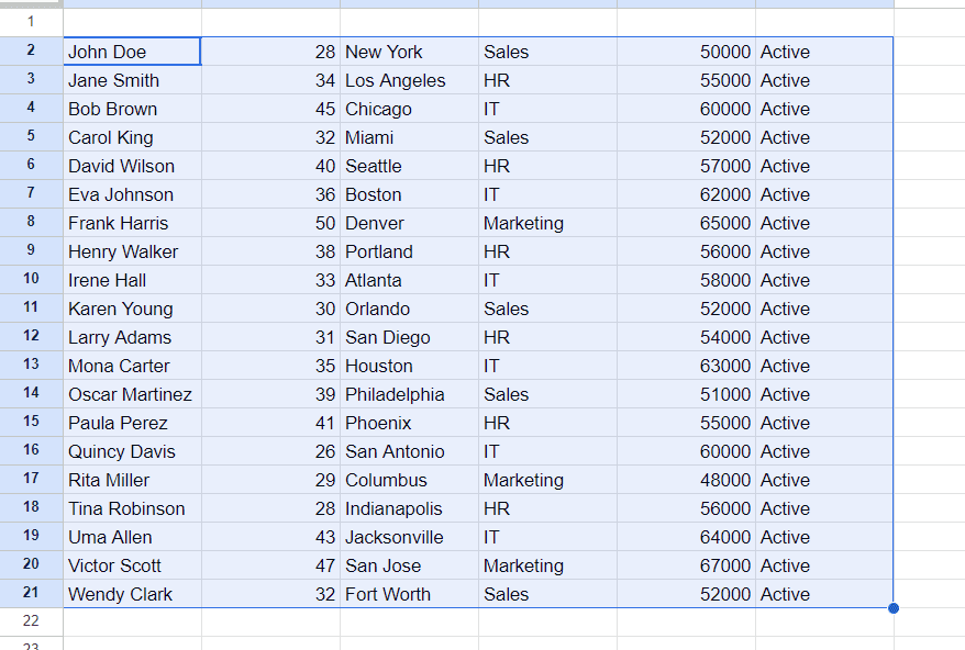
By following these simple methods, you can easily copy only visible cells in Google Sheets, avoiding the inclusion of hidden rows and columns.

This technique is invaluable for maintaining clean and relevant datasets, ensuring your reports and consolidated sheets contain only the information you need.